Advanced Conditional Formatting

Welcome back, spreadsheet maestros! You’ve already gotten a taste of how to make your data shine with basic conditional formatting, but today, we’re kicking it up a notch. We’re diving into some more advanced techniques that will take your spreadsheets from good to great. Ready? Let’s get started!

Coloring an Entire Row Based on a Condition

Sometimes, highlighting just a single cell isn’t enough. You may want to draw attention to an entire row when a condition is met, such as when a task is overdue or when a customer’s order needs follow-up. Thankfully, Google Sheets makes this easy with the right custom formula.

Example Scenario:
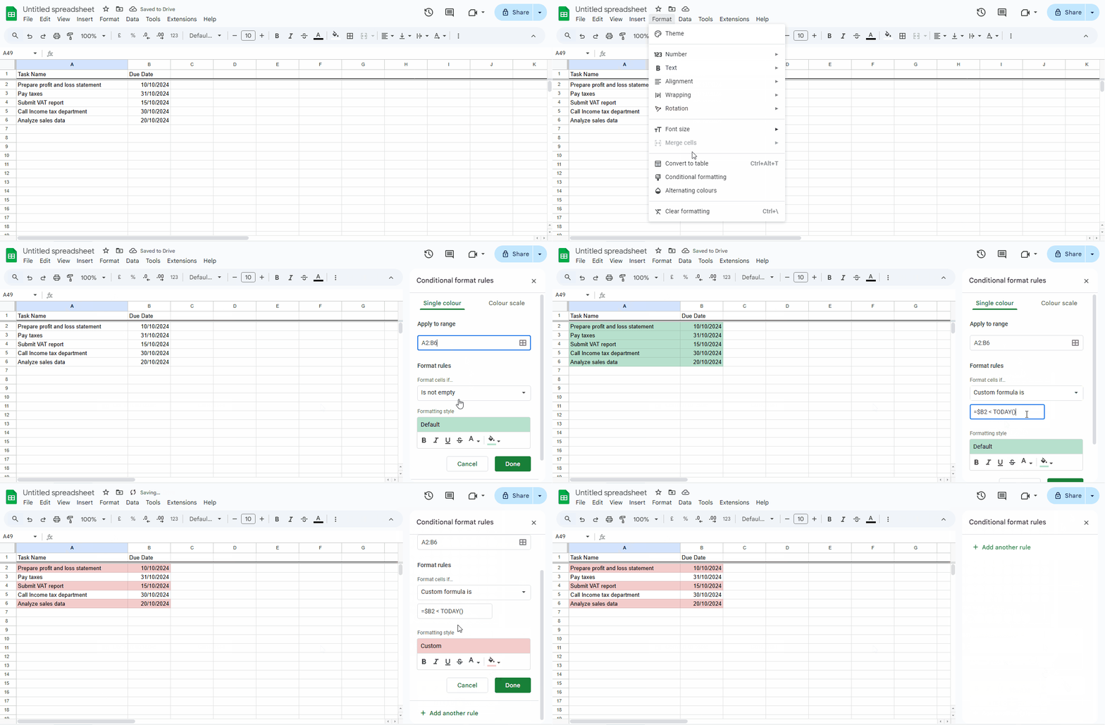
Suppose you have a list of tasks in your spreadsheet. Column A contains task names, and Column B contains due dates. You want to highlight the entire row in red if a task is overdue.

Here’s how you do it:

1. Select the range of rows you want to format.

2. Go to Format > Conditional Formatting.

3. Choose “Custom formula is” from the drop-down menu.

4. Enter this formula:

5. Pick a red fill color and click “Done.”

Explanation:
The formula checks if the date in Column B (due date) is less than today’s date, meaning the task is overdue. By using $B2, you ensure that the condition checks Column B for every row, and the $ sign locks the column so that it doesn’t shift when the formula applies to the rest of your range.

Understanding the Magic of the $ Sign

When using custom formulas, the $ sign is your best friend. It helps you control which parts of the formula stay fixed and which parts can change. Here’s a quick breakdown:

• Without the $ sign: The formula adjusts both the row and column as it moves across the range.
• With $ before a letter (e.g., $A1): Locks the column (A stays A) while the row can change.
• With $ before a number (e.g., A$1): Locks the row (1 stays 1) while the column can change.
• With $ before both (e.g., $A$1): Locks both the row and the column, so the formula will always refer to cell A1.

More Examples Using Custom Formulas

1. Highlighting Entire Rows for Specific Values

• Let’s say you have a customer order list. Column C contains the status (“Completed,” “Pending,” or “Cancelled”). You want to highlight all “Cancelled” orders in light gray.

Formula:

Why it works: The $C2 locks the formula to check only the value in Column C for each row.

2. Coloring Rows Based on Multiple Conditions

• Imagine you’re running a survey, and you want to highlight responses where the age (Column B) is over 30 and the satisfaction score (Column C) is below 3.

Formula:

Why it works: The AND function lets you combine multiple conditions. Both need to be true for the row to be highlighted.

3. Dynamic Highlighting Using Multiple Columns

• Suppose you want to highlight rows where the sales team hit their monthly target. Column D has the target, and Column E has the actual sales. Color the row green if the sales in Column E are greater than or equal to the target in Column D.

Formula:

Why it works: The formula compares the value in Column E to Column D for each row, and the $ locks the columns so the comparison remains consistent.

Practical Tips for Using Advanced Conditional Formatting

• Use Custom Formulas Wisely

Custom formulas give you a lot of flexibility, but they can also get complex. Start simple, and test your rules on a small sample to ensure they work as expected.

• Layering Multiple Rules

You can add more than one conditional formatting rule to a range. For example, you might color rows green when sales targets are met, red when they’re missed, and yellow when they’re close.

Make sure to arrange the rules in order of priority, as Google Sheets applies them sequentially.

• Copy and Paste Conditional Formatting

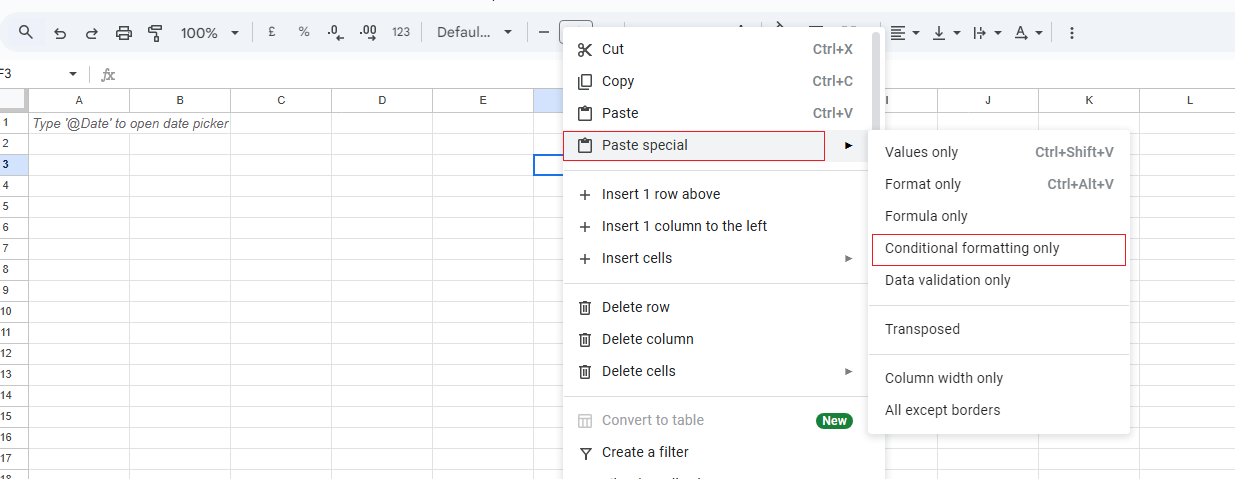
Did you set up a beautiful formatting rule but need to apply it elsewhere? No problem! You can copy the cell with the rule, then right-click and use “Paste Special > Conditional Formatting Only” to apply it to other cells.

Wrapping Up: Level Up Your Google Sheets Game

Conditional formatting can transform how you view and analyze your data. Whether you’re managing projects, tracking sales, or just keeping tabs on your favorite sports team, these advanced techniques give you the flexibility to see what matters most, instantly.